


TL;DR: Microscopy AI models must be evaluated against simple baselines to understand when they are learning genuine biology or exploiting technical shortcuts like cell density or pixel intensity. While the field is shifting toward massive foundation models, a few benchmarks reveals that some networks often capture similar biological signal as untrained models, even when the biological signal is significant. While massive, in-domain models can successfully capture subtle phenotypes, interpretable baselines are needed to contextualize their true capabilities. To further advance drug discovery, we must make performance interpretability a core design of our benchmarks.
Connect with us: Valence is constantly seeking talented individuals with diverse backgrounds and expertise to join our team. Explore open roles here.
The complexity of the image produced by a microscope is often underappreciated.
When taken out of context, it is just an image of cells. But, in the context of a perturbation experiment, it contains more information: it shows how cells transform when some gene is perturbed or a chemical compound is added. It captures changes to the cell’s features like its shape, texture, intensity, spatial distribution of organelles, and overall arrangement.
This explains the growing importance of microscopy as a major source of phenotypic data in drug research and development. This data allows the researcher to analyze large amounts of experiments and observe different properties of the cells: toxicity, mechanism of action, cellular state, response to stresses, and activity pathways.
While some of this information is invisible to a human analyst, much of the information is rather subtle : only statistically significant after comparing large numbers of samples and many microscopic fields of view.
This is precisely where deep learning comes into play.
Part of my own interest in this question comes from some of my prior work benchmarking single cell transcriptomics models. In that setting, I have repeatedly seen that impressive benchmark numbers can look less impressive once they are compared against simple but well-chosen baselines. A model may appear to understand biology, when it is partly exploiting batch effects, dataset structure, cell-state prevalence, or other shortcuts. That experience made me wonder how much of the same story applies to microscopy.
The power of neural networks for natural image analysis is well-understood. Neural networks are increasingly used in several fields of life science research, including transcriptional profiling and histological pathology analysis. Transcriptional profiling and histological pathology analysis share similarities with microscopy imaging: the former relies on matrices of gene expression data while the latter uses images of tissue sections. Further, like transcriptomics, microscopy can answer questions like: what happens to the biology upon perturbation?
We’ve moved beyond asking whether microscopy images contain biological signals, we know they do. The harder question, and the one I care about most as a benchmarker, is whether our models, and our benchmarks, can tell us what part of the biological signal they have learned.
The type of biological imaging we refer to
When “biological imaging” is mentioned, usually people think about histopathology with stained tissues, cancer diagnosis, and clinical pathology. This is an important branch in biology, and it has been a focus of the machine learning community.
However, the area we refer to is something quite different. We speak about preclinical microscopy imaging: Cell Painting, brightfield imaging, high-content screening, and large scale cell perturbations.
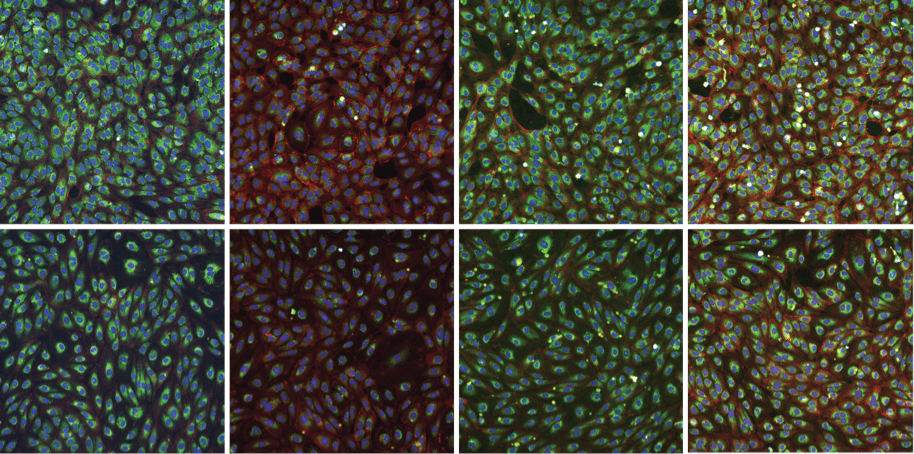
Figure 1 : RxRx1 Cell Painting images
Cell Painting is perhaps the best example to explain our topic. Here, cells are treated with a limited number of fluorescent probes, which stain cellular components. As a result, we can identify the nuclei, mitochondria, endoplasmic reticulum, actin cytoskeleton, Golgi apparatus, ribonucleoprotein granules and other morphological landmarks. This technique does not help us analyze individual markers. Instead, it allows us to obtain a complete phenotypic profile for each cell.
For instance, in a typical high content screen, thousands of drugs or genetic modifications can be tested in various plate conditions, then imaged and computationally analyzed for their phenotypic similarity. Thus, if two drugs create a similar profile, we can infer that they work through a common molecular mechanism. Likewise, phenotypic alignment between a gene knockout and a drug can identify the drug’s potential target. Finally, any particularly robust or unique phenotypes uncovered by these screens serve as high-priority candidates for downstream investigation.
This is a simple idea with large implications: instead of measuring only whether a cell lives or dies, we can measure how the cell changes and use that information to infer potential targets and / or treatments.
From handcrafted morphology to foundation models
While the first generation of image-based profiling did not require deep learning, it required intensive image analysis.
Thanks to tools like CellProfiler, cells could be segmented and annotated based on image morphology, including size, shape, texture, intensity, granularity, radial distribution, and much more. This transformed the cell from an image into tabular data, allowing for applications of bioinformatic methods including: normalization, quality control, aggregation, similarity search, clustering, and statistics.
This was an important milestone. It enabled computability of microscopy images. At the same time, no deep learning was needed to analyze cells. The feature space was pre-defined, interpretable, and powerful enough to sustain years of morphological profiling.
Handcrafted features had their own limitations, though. They could only reflect patterns that we knew how to extract. There might exist biological patterns which are real, reproducible, and meaningful, yet impossible to encode using a conventional texture or shape descriptor.
That is where machine learning came into play. Instead of specifying the features that one must analyze , machine learning algorithms can be trained to learn the relevant representation of data automatically.
The evolution of our methods followed a predictable path. At first, there were specialized image-based CNNs, followed by models trained under weak supervision for perturbation or experimental label prediction. Most recently, the field moved towards self-supervised and foundation models: large-scale neural networks trained on vast microscopy datasets and applied to different downstream tasks.
The promise is attractive. All in all, such a microscopy foundation model would allow us to overcome many limitations of handcrafted feature-based approaches. It could serve as a universal feature extractor for biological images, streamline profiling workflows, improve perturbation retrieval, facilitate MOA discovery, and open up image-based profiling to people without the ability to construct a computer vision pipeline.
On the whole, the ambition looks pretty similar to what happened in the field of natural image understanding. A trained model becomes useful due to having learned reusable patterns of data: starting from edges, textures, and object parts, moving up to higher-level scene semantics.
This was ported over to microscopy data. Given that the key advantage of this data is that it is scalable (if a method has been standardized, then it allows us to collect very large phenotypic datasets with relative ease), this made it prime grounds for scaling deep learning applications in drug discovery.
However, scale also changes the practical shape of the field: who can train these models, who can evaluate them properly, and who can reproduce or challenge the conclusions.
Size of the Dataset: To begin , datasets in the microscopy field are gigantic. Of course, transcriptomics datasets are often big as well, however, transcriptomic datasets typically involve a relatively sparse matrix of genes and cells. Microscopy datasets consist of images in one or more channels across many plates, sites, and fields. Public Cell Painting resources can go as high as hundreds of terabytes. And industrial datasets can go far higher than that. This means a significant shift of who is allowed to join the party. One can just download a transcriptomics dataset onto a laptop computer and analyze it locally. Trying to pull a big imaging screen off the server and process it is a totally different beast. This is not an argument against scale. In fact, microscopy is one of the areas in biology where scale has clearly mattered. The issue is that the same scale that enables strong representations also makes careful benchmarking expensive, both at training time and at inference time. That creates a need for smaller but representative benchmarks, precomputed embeddings, and curated subsets that let more laboratories participate.
Experimental Protocol: Microscopy experiments depend quite a bit on the particular setup and conditions under which they are performed. Things like the microscope, staining protocols, plate format, cell density, image focusing, illumination, batch, vendor, and acquisition settings are all factors that influence the way an image is collected. Some of these effects are biological, others technical, some both. It’s easy for a model to train on specific characteristics which will not generalize to other collections.
Interpretability: Gene names are intuitive. There’s even literature associated with pathways and protein interactions. Image embeddings, on the other hand, are not. It could be true that a model knows something meaningful about the differences between two perturbations from their images, but the researcher still wants to know what that is.
There have been big changes in recent years that have helped us overcome all three of these challenges.
Publicly available data sources like JUMP-CP and the Cell Painting Gallery have allowed us to think more clearly about the scale needed for modern representation learning, with efforts to reduce dataset size while retaining the same number of samples and performance. The availability of large-scale industry datasets has accelerated this trend.
There have also been architectural advancements that have made microscopy-focused modeling possible. Channel-adaptive or channel-agnostic modeling is an essential example. Models for natural images assume three input channels: red, green, and blue. Microscopy works differently. Some assays use one brightfield channel. Other assays use five fluorescent channels. Yet another may use a different number or combination of these channels with a different order. The useful model would need to be flexible to different configurations of the channels.
That’s where channel-agnostic masked autoencoders and their DINO analogs come in. It’s not merely a matter of techniques but a matter of embedding the biology of microscopy and its experimental reality into foundation models.
And of course, there’s scale. With larger models being trained on larger microscopy data collections, we can get better representations, particularly with training and evaluation data similar to our downstream biological task. It means that some of the scaling effects that have proven successful in natural image and language models are genuinely relevant in microscopy too.
But a key question has surfaced after all these advancements : What have the microscopy models actually learned?
Benchmarking what models really learn
A benchmark score is valuable only insofar as we understand what it proves.
On natural images, a good performance on ImageNet typically indicates that the model has developed a representation of visual features suitable for object recognition. While this is by no means a perfect benchmark, decades of scrutiny have helped to elucidate many of its failings.
Benchmarks in microscopy are far newer, though there have been many successful efforts improving these in different academic and industrial contexts.
One useful benchmark, proposed in recent microscopy benchmarks, is to ask whether a representation can recover known biological relationships. In practice, perturbations are embedded, ranked by similarity, and evaluated by how well they retrieve known relationships such as shared mechanism of action, gene function, pathway membership, or other curated biological links. This kind of recall is useful because it is closer to the scientific question than ordinary classification accuracy: do phenotypes that should be biologically related end up close to one another?
This gives us a concrete starting point for asking whether a model is organizing images according to biology, rather than merely exploiting nuisance variation.
The question now is what additional diagnostic baselines can tell us about what drives a score in these benchmarks.
There is no denying that the model has learned biological morphology, which is exactly the intent in the field. However, the model has the possibility of also learning biological intensity statistics, biological cell density, biological plate layout, biological acquisition bias, biological stains, biological focus statistics, or biological dataset structure. All of these can contribute to the benchmark score, although it does not necessarily imply biological abstraction.
A robust model ought to be compared not only against other trained models, but against simpler baselines. How much information can be learned about biological samples from pixel intensities alone? What can be learned from cell counts alone? Can a biological signal be extracted from an untrained neural network? How much information about structure can be inferred independent of image intensity? Simple as they might seem at first glance, these benchmarks serve to demonstrate how much of the task can be solved independent of the desired learning capability. These baselines help distinguish performance that reflects reusable biological structure from performance that reflects shortcuts specific to the benchmark.
Comparing a trained model against weak baselines yields little insight. Against powerful diagnostic baselines, however, the model will reveal plenty.
That is the problem my collaborators and I examine in our new paper, Deep Learning for BioImaging: What Are We Learning? seeks to explain at ICML 2026. I should be explicit about my position here: I work at Valence Labs @ Recursion, and one of the strongest-performing models discussed below comes from our own work. But the point is not simply to show that a larger in-domain model performs well, but use it as a reference to ask what kind of biological evidence this performance reflects.
The paper examines representation learning in bioimaging over two scales of imaging: cell culture microscopy and tissue imaging. Rather than simply asking which model scores highest on the given benchmark, the work asks what this score represents.
To do so, the paper re-examines existing benchmarks through the use of very simple yet insightful baselines:
In cell culture microscopy, trained microscopy models are compared with untrained neural networks and pixel-statistics features.
In tissue imaging, image foundation models are compared with structure-only representations derived from cellular organization.
These baselines are intentionally unambitious. They do not aim to propose novel foundation models. Rather, they aim to reveal the limitations of the benchmarks themselves.
The results are telling.
In a few cell-culture microscopy tasks, multiple trained models perform rather similarly to untrained and extremely simple baselines. The implication is clear : part of the benchmark signal does not require high-level biological representation learning. Architectural bias and low-level image statistics alone contain enough information in many instances.
At the same time, the largest in-domain model we evaluate, the MAE-G/8 model is clearly above these baselines on the evaluated tasks. I think the cautious interpretation is : scale, in-domain biological data, and the training recipe appear to add information beyond obvious low-level confounders, but the baselines help clarify where that extra information is actually needed.
In other tasks, especially those where the biological signal is either more subtle or better aligned with the pre-training data, in-domain foundation models show their benefits compared to simple baselines. The takeaway is that benchmark scores should be calibrated to the specific task by using biologically interpretable and informative baselines for comparison.
A model’s performance might incorporate various components: true biological information, useful visual priors, technical correlations, and domain-specific shortcuts where the presence of specific biological components can be correlated to the outcome of a specific downstream task and not another.
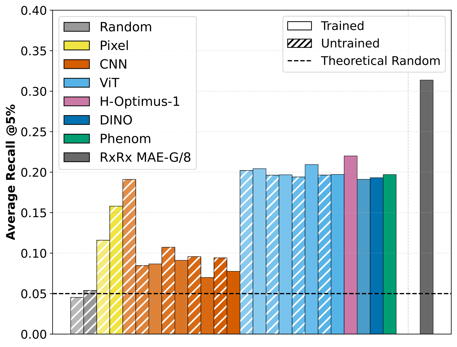
Figure 2 : Average recall of known biological relationships on rxrx3-core benchmark of different pretrained models vs untrained model weights.
For me, as both a model builder and someone who cares about benchmarking, this says something simple: there is no roadblock in front of us. Models are succeeding on different downstream tasks. What is still missing is a sharper set of interpretable tools for measuring what they have learned, when they should be trusted, and which model is appropriate for which downstream task.
If a simple baseline performs well in solving a given task, it’s a piece of information about the task, its requirements, and what kind of evidence is required for claims that a given model learns reusable biological structures. And, more importantly, it’s a valuable insight on how to build a benchmark properly. Namely, in order to test deep representation learning ability, it should include measurements that separate correlations from the underlying biological signal.
At the core of our approach is a single concept: advances in microscopy representation learning need better interpretability, both at the model level and at the downstream task level.
It tells us if representations can be generalized between experiments. If morphological information was captured without density features. If a foundation model did learn subtle phenotypes.
Implications for the field
What’s next for deep learning in microscopy research? Scaling up has been shown to be a successful recipe, especially when trained with high quality data. What is missing is a more mature interpretability and explainability culture.
There are a number of directions that would accelerate practical deep learning applications for impact :
Accessible datasets are needed. Currently, many of the largest-scale imaging screens are simply too big to be handled by ordinary laboratories. Compressed benchmarks, curated subcollections, precomputed embeddings, and cloud-native tools are all necessary steps. But accessibility is also essential. It allows new participants to emerge. Whether it is through crops, smaller image sizes, or data deduplication, we need to find how to preserve good model performance while avoiding the massive memory overhead of microscopy imaging data. Several works are going in this direction.
Baselines need to become more portable and more routine. The next step is to make such comparisons easier to run for new datasets and new tasks: using pixel statistics, cell counts, feature engineering, plate information, structural information, and precomputed embeddings where possible. This should not be seen as a secondary consideration. Baselines are integral to interpretation and adoption.
Interpretability needs improvement. Here, it should not be assumed that every learned feature corresponds to a well-defined biological concept. That is not always true for biology. However, biologists will still need ways of connecting image-based features to morphology, pathways, mechanisms, quality assessment, and experiments. A good microscope model is more than an embedding.
Usable software is essential. What allowed CellProfiler to revolutionize microscopy was, in part, its accessibility. Deep learning applied to microscopy will also need that spirit: models that are easy to use as tools; embeddings that easily integrate into workflows; documentation written for biologists; and benchmarks accessible to graduate students without their own specialized infrastructure.
This may be one of the most profound takeaways from the history of bioinformatics. A technique is powerful if and only if it becomes integrated into normal scientific practice.
One may call microscopy an underdeveloped cousin of transcriptomics, and in a certain sense, it is true. Transcriptomics boasts standardized data formats, mature statistics, and straightforward transition from feature vectors to biological interpretations.
Yet microscopy has something else: phenotypes, spatial arrangements, scalability, industrial use, and potential to uncover phenomena not amenable to molecular interpretation.
The point is not to pit the two against each other. The most effective biology ML models will likely incorporate all types of input data : gene expression, morphology, chemical structures, proteomics, spatial relations, and existing biological knowledge. And all modalities are bound to have gaps in their coverage of biological phenomena. At the same time, they will show the same reality from different perspectives.
This makes microscopy essential for the future of biological ML models because of its ability to capture not what a cell holds but who a cell is.
Yet for that perspective to work well, we should understand what machine learning algorithms see when they analyze microscopic images.
This post is part of “Inside Valence”, a series where you’ll get a behind-the-scenes look at our research, exploring new ways to predict, explain, and ultimately decode biology. If this resonates, consider subscribing!
 | A guest post by
|